R Statistics

 Module 7: S3 and S4 I did what I could do and I am taking more time to understand how that the object oriented side of R works. I was very confused on this entire Module, but since that this is crucial information, review on my own time is how I see to remedy my lack of understanding. I saw that the assignment was due at 8PM instead of AM, I was not sure and decided to try as hard as I could until the end to understand what to do, when, why and how.  Questions: 1) S3 is quite generic and plain and is more of a 'one at a time' format where S4 has more formal classes that are inheritable and also can analyze and choose input from an array of arguments instead of a singular argument like S3 2) Using functions like class(), typeof() and even str() can help a user find out information about a dataframe 3) Generic Functions are like a universal, one size fits all type of function that can take a wide variety of input types and generate results.  4) As stated in question 1, differenc

 This is my Module 7 Assignment for Data Distributions in R, I decided to use ggplot and take this in a slightly different direction by introducing Kernel Density Distributions as my chosen trendline on a series of histograms to see what kind of information can be found based on the density of sample member values in particular categories in the MTCARS dataset built into R. I submitted a compiled RMarkdown HTML File in Canvas since for the life of me I could not find a way to import it to blogger :(

Module 6 Assignment Another attempt at using R correctly, and as a special treat, I decided to painstakingly enter all values for the last problem for that matrix, because I could not figure out how to properly use diag() to do it. ##Module 6 Doing Math Part 2 #Build and Save two matrices as outlined in the instructions A <- matrix(c(2,0,1,3),ncol = 2) B <- matrix(c(5,2,4,-1),ncol = 2) A B #Find A + B addmatrix <- A + B addmatrix #Find A - B submatrix <- A - B submatrix ##Problem 2 Use diag() to create a size 4 matrix with values 4,1,2,3 in the diagonal diagmatrix <- diag(x = c(4,1,2,3)) diagmatrix ##Problem 3 deconstruct a matrix into code sequence p3 <- matrix(c(3,2,2,2,2,1,3,0,0,0,1,0,3,0,0,1,0,0,3,0,1,0,0,0,3), nrow=5, byrow=TRUE)

 Module 5: Doing Math ##Module 5: Doing Math ##Your Assignment: #Find the value of inverse of a matrix, determinant of a matrix by using the following values: #  A=matrix(1:100, nrow=10) #  B=matrix(1:1000, nrow=10) #  Post your result and procedure you took on your blog. #  A good start will be: #    >A <- matrix(1:100, nrow=10)   #  >B <- matrix(1:1000, nrow=10) library(dplyr) library(Matrix) library(matlib) install.packages("matlib") #The instructions are posted above, but lets get started by identifying the first step: Finding the Inverse of the Matrix ##Lets start with Matrix A a <- matrix(1:100, nrow = 10) View(a) ##Let's generate the inverse of the matrix solve(a) det(a) #Matrix B b <-matrix(1:100, nrow = 10) Inverse(b) det(b) # Both determinants ended up being zero, but both methods of inverting the matrix spun an error message because that the matrix #is a non singular matrix, in the case of both a and b

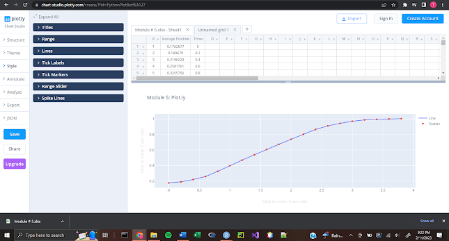
 Module 5: Plot.ly This weeks assignment consisted of toying about with a software called Plot.ly. I like to think this is a slightly more user friendly and comparable interface to Tableau at which with the provided dataset I was able to visualize a scatter and line graph that correspond to one another by using two trace layers in my assignment. The outcome is based on how expansive the data is but, this data was only two columns, which calls for a simpler visualization. 

  My results were a bit rudimentary and odd. More than my results, what kind of data slicing was necessary for this homework assignment, and furthermore, do you have any good advice on how to be more creative with tableau, this is my first time ever hearing about or using this software, so I am a bit lost but I am still eager to learn. I sliced the variables down to the most sensible based on their amounts, the hard part is accurately visualizing them because there are some values that are lower end outliers, where they are far less than the others by an magnitude base order of ten, some numbers are millions, and some are in the billions on this visual. What I am curious to know, is how that us students can locate and find more in app elements to assist with our creation of these visuals.

 ##Module 4 Programming Structure in R ##First things first, lets call in some libraries that would be of great use to us library(dplyr) library(ggplot2) library(tidyverse) #Now, lets define all of the data provided in the instructions frequency <- c(0.6,0.3,0.4,0.4,0.2,0.6,0.3,0.4,0.9,0.2) BP <- c(103,87,32,42,59,109,78,205,135,176) first <- c(1,1,1,1,0,0,0,0,NA,1) second <- c(0,0,1,1,0,0,1,1,1,1) finaldecision <- c(0,1,0,1,0,1,0,1,1,1) mydata <- data.frame(frequency,BP,first,second,finaldecision) #Lets calculate the mean of the Final Decisions ratings using mean() ##We will make this a variable called "FinalDMean" FinalDMean <- mean(mydata$finaldecision) ##Now lets clean the data by replacing the NA value in 'first' with a zero mydata$first[is.na(mydata$first)] <- 0 View(mydata) #Now that the data is all nice and tidy, lets enable ggplot for the boxplots and histograms, I am using this package in another class ##Might as well keep using it si